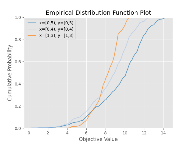
plot_edf

optuna.visualization.matplotlib.plot_edf(study, *, target=None, target_name='Objective Value')

Matplotlibを使用して、スタディの目的関数値EDF（経験分布関数）をプロットします。

EDFをプロットする際には、完了したトライアルのみが考慮されますのでご注意ください。

See also

使用例については optuna.visualization.plot_edf() を参照してください。 この関数は同機能を持つ optuna.visualization.plot_edf() で置き換え可能です。

Note

生成される凡例のスタイルを調整するには、matplotlib.pyplot.legend のドキュメントを参照してください。

Parameters:

• study (Study | Sequence[Study]) – 対象とする Study オブジェクト。 複数のスタディを指定して、それぞれのEDFを比較することも可能です。

• target (Callable[[FrozenTrial], float] | None) –

  表示する値を指定する関数。None を指定し、study が単一目的最適化に使用されている場合、 目的関数値がプロットされます。

  Note

  study が多目的最適化に使用されている場合は、この引数を指定してください。

• target_name (str) – 軸ラベルに表示する対象の名称。

Return type:

Axes

The following code snippet shows how to plot EDF.

/mnt/nfs-mnj-hot-99-home/mshibata/sandbox/optuna-documentation-plamo-ja/optuna-doc-plamo-translation/tmp-optuna/docs/visualization_matplotlib_examples/optuna.visualization.matplotlib.edf.py:43: ExperimentalWarning:

plot_edf is experimental (supported from v2.2.0). The interface can change in the future.


<Axes: title={'center': 'Empirical Distribution Function Plot'}, xlabel='Objective Value', ylabel='Cumulative Probability'>

import math

import optuna


def ackley(x, y):
    a = 20 * math.exp(-0.2 * math.sqrt(0.5 * (x**2 + y**2)))
    b = math.exp(0.5 * (math.cos(2 * math.pi * x) + math.cos(2 * math.pi * y)))
    return -a - b + math.e + 20


def objective(trial, low, high):
    x = trial.suggest_float("x", low, high)
    y = trial.suggest_float("y", low, high)
    return ackley(x, y)


sampler = optuna.samplers.RandomSampler(seed=10)

# Widest search space.
study0 = optuna.create_study(study_name="x=[0,5), y=[0,5)", sampler=sampler)
study0.optimize(lambda t: objective(t, 0, 5), n_trials=500)

# Narrower search space.
study1 = optuna.create_study(study_name="x=[0,4), y=[0,4)", sampler=sampler)
study1.optimize(lambda t: objective(t, 0, 4), n_trials=500)

# Narrowest search space but it doesn't include the global optimum point.
study2 = optuna.create_study(study_name="x=[1,3), y=[1,3)", sampler=sampler)
study2.optimize(lambda t: objective(t, 1, 3), n_trials=500)

optuna.visualization.matplotlib.plot_edf([study0, study1, study2])